Expeditions
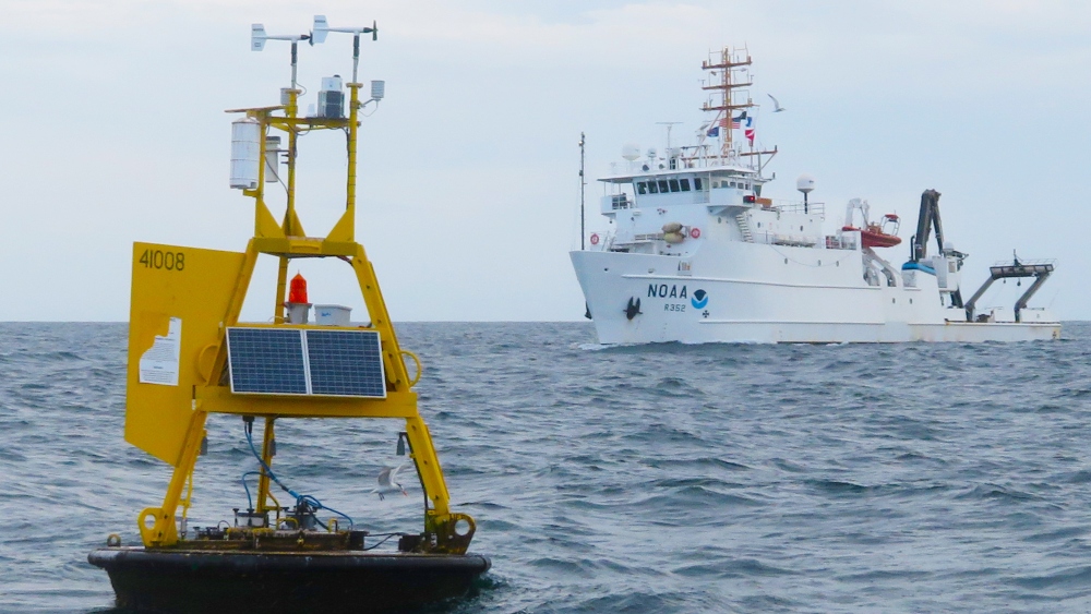
Each year, Gray's Reef applies for ship time on board one of the NOAA ships to conduct expeditions in and around the sanctuary. Mainly using the NOAA Ship Nancy Foster, Gray's Reef science staff coordinate expeditions usually lasting several days to several weeks. Science partners submit research proposals to conduct research in a number of scientific disciplines. Gray's Reef staff also participate in expeditions aboard other vessels and in other areas.
View the sanctuary's science needs assessment.
2023
A two-leg mission focused on exploring live-bottom habitat on the eastern continental shelf through scuba diving and seafloor mapping. A team of 12 researchers completed the 15-day mission (June 14–July 1). The expedition projects explore:
- multibeam bathymetry mapping
- seafloor and ledge characterization
- focal species surveys
- photo and video transects
- fish identification for diversity and abundance
- drop camera surveys
2022
A team of 12 researchers collected scientific data from the sanctuary for an 11-day mission (July 7-17). The expedition projects explore:
- multibeam bathymetry mapping
- fish abundance and distribution
- macroalgae diversity
- invertebrate assessments
- single-celled organism assessments
- water and sediment microplastics collection
- microbial communities that live symbiotically with the reef's resident macroalgae
- invasive lionfish survey and removal
2021
Leg Mission I Objectives:
A mission dedicated to seafloor mapping, a sanctuary scientist joined Nancy Foster survey technicians and mapped 43 square miles of seafloor southeast of the sanctuary during an eight-day mission (May 26–June 2).
- multibeam bathymetry mapping
- ocean current profiling and water movement
- day-night fish and plankton changes
Leg Mission II Objectives:
This nine-day expedition (August 7–15) explored the following topics about the sanctuary:
- multibeam bathymetry mapping
- fish abundance and distribution
- macroalgae diversity
- single-celled organism assessments
- water and sediment microplastics collection
- microbial communities that live symbiotically with the reef's resident macroalgae
- invasive lionfish survey and removal
2019
Mission Objectives:
A nine-day expedition (July 29–August 9) explored the following topics about the sanctuary:
- multibeam bathymetry mapping
- fish abundance and distribution
- macroalgae diversity
- invertebrate assessments
- the structural habitat of Gray's Reef
- microbial communities that live symbiotically with the reef's resident corals
- invasive lionfish survey and removal
2018
Mission Objectives:
The expedition explored these topics during its 10-day mission (July 30–August 8):
- biodiversity "hot spots" on ledges
- fish predation ecology
- coral stressors
- macroalgae diversity
- reef bio-physical interactions
- seafloor water chemistry monitoring
- coral larvae collection
- microbial communities that live symbiotically with the reef's resident corals
2017
Mission Objectives:
An extended 15-day mission (June 9–23) explored these research projects in Gray's Reef National Marine Sanctuary:
- fish predation ecology
- macroalgae diversity
- invertebrate assessments
Additional expedition reports are available upon request. Email graysreef@noaa.gov for more information.